Survival Analysis – Statistical methods and how we can use them for effective decision making

What is survival analysis?

Survival Analysis is a relatively under-utilized set of statistical tools, which addresses questions such as ‘how long would it be before a particular event occurs’. Therefore, sometimes it is also said to be ‘time to event’ analysis.

Why the term “survival”? This is because the method was developed by medical researchers who were interested in finding the expected lifetime of patients in different cohorts (ex: Cohort 1- treated with Drug A & Cohort 2- treated with Drug B).

This analysis can be further applied to different types of events of interest in different business domains. Take Netflix for instance. One can use survival analysis techniques to estimate how long a particular customer stays subscribed. It can then help the marketing team to devise strategies to retain them so that the business stays healthy.

Hence, broadly speaking “Survival Analysis is used to analyze the expected amount of time for an event to happen”.

What problems can be addressed/solved?

Any statistical method, without real-life applications, is useless. So, let’s take a look at some of the use cases where survival analysis can really land a punch.

• How long can a business expect a customer remain subscribed to its content?
• The expected lifetime of people taking a pharmaceutical drug
• Effectiveness and comparison of different marketing campaigns
• Reliability analysis of machine equipment i.e. how long will it take for machine equipment to function to fracture/fail

Mathematical Definitions

As with any field of mathematics, there are some terms that need to be understood clearly before going further. Also, it helps if these terms are explained with the help of a use-case.

Consider the classical Cohort Analysis problem where different cohorts are behaviorally compared and evaluated against certain metrics. Suppose you want to track the behavior of three cohorts (A, B & C) and the metric is retention rate.

Here,

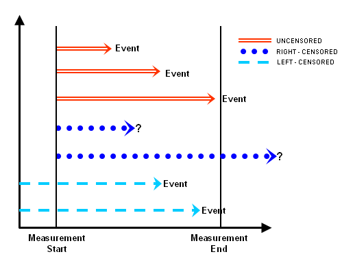
Event: Time at which the customer unsubscribes a marketing channel
Time of origin: Time at which the customer starts the service/subscription of a marketing channel
The time scale could be days/weeks/months depending on the situation.
Basically, you want to model the “time-to-unsubscribe” event.

Need for survival analysis

You might be asking yourself this question “Can’t we take the average of ‘event’ times (during the observation period) and compare?”

However, as it turns out (and this is going to be true), there are going to be customers who are still subscribed and these data points (customers) are said to be “right-censored”. There’s another type of censored data called “left censored” where the birth event is unknown. In the explanations below, we will be only dealing with right-censored data.

‍Fig: Censored Data in a study

It simply means that we haven’t observed the “event” for them. Taking the average would simply result in underestimation of the true time-to-event statistic; in your case, you might be under-estimating the retention rate.

Survival analysis gives us a way of using the information of right-censored data points to inform the model. It is more useful than simply averaging time to event for only those who experienced the event.

Mathematical Intuition of survival analysis

Assume a non-negative continuous random variable T representing the time-to-event of interest. In our example, it is the time-to-unsubscribe for cohorts. Since T is a random variable, we can define its PDF (probability density function) and CDF (cumulative density function). Let’s take its PDF as f(t) and CDF as F(t).

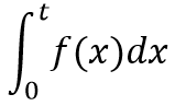
1. F(t) – It can also be denoted by P(T<t) and gives the probability that the event has happened by time t. If we look at its integral form, we can see that it represents the proportion of the population with time-to-event less than t.

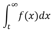
2. Survival Function: Mathematically, it is written as S(t) = 1 – F(t) = P(T>=t). It gives the probability that the event hasn’t occurred by time t and gives the proportion of the population with time-to-event value more than t.

3. Hazard Function: It is defined as the probability that the subject will experience an event of interest within a small time interval, provided that the individual has survived until the beginning of that interval. In simple terms, the higher the hazard in a time interval, the higher are the chances of the event happening. Mathematically it is denoted by h(t) = f(t)/S(t).

Kaplan Meier Estimate

The starting point of the analysis is to capture the PDF which is then used to model the survival function. Oftentimes we won’t have the true survival curve of the population and is estimated by two ways- parametric and non-parametric.

The first method assumes a parametric model, which is based on certain distributions (ex: exponential distribution), then we estimate the parameter, and then finally form the estimator of the survival function.

A second approach is a powerful non-parametric method called the Kaplan-Meier estimator. We will discuss it in this section.

Below defined is the survival function for the Kaplan-Meier method. Here,

ni: the population at risk at the time just prior to ti

di: number of events occurred at time ti

Mathematically, the area under the KM curve gives the expected lifetime. And the median lifetime is the time (X-axis coordinate) at which y=0.5.

Python implementation using “lifelines” package

Now, we’ll be using the “lifelines” package to code things up. You can explore more of it here. Keeping in sync with the cohort analysis example, we’ll try to compare the retention rates of cohorts obtained from the Telco-Customer churn dataset which can be found here.

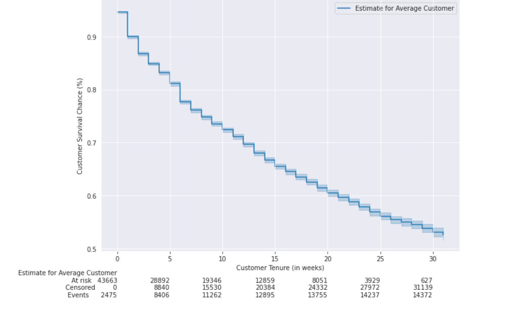
First, let’s plot out the overall KM survival curve with data frame df:

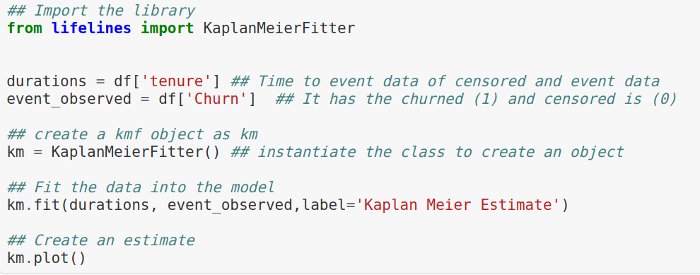
It produces the following plot:

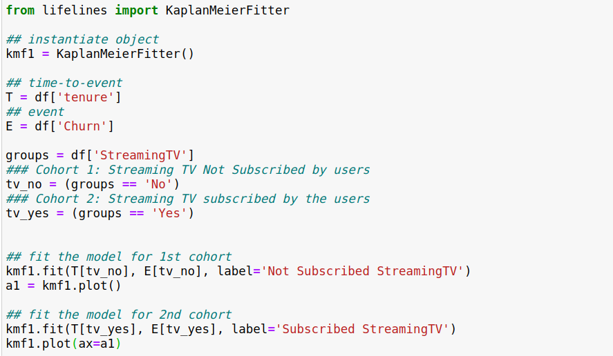
Now, we will compare two cohorts: One which subscribed to Streaming TV and the other didn’t.

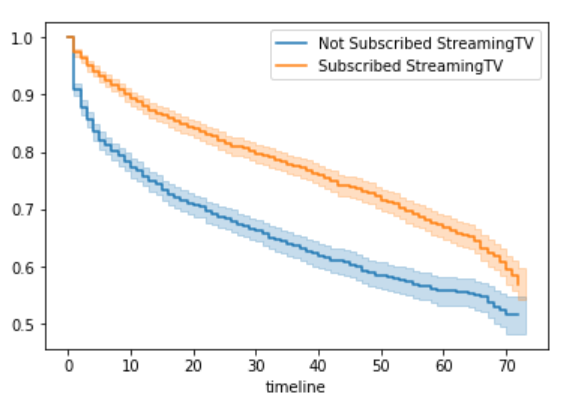
From the plot above, it is evident that the customers, who have subscribed for the Streaming TV (orange), have better customer retention as compared to the customers, who have not subscribed for the Streaming TV (blue).  Also, their confidence intervals (width of lines) do not overlap and are low width, hence we can guarantee its statistical significance (check out the logrank test in lifelines package to validate this), i.e. these two curves are statistically different.

Conclusion

This is only the beginning of a vast field of mathematics. There are other interesting things to explore like parametric regression, non-parametric regression, accelerated failure time models, etc. Even deep learning-based survival analysis is being carried out nowadays. You can check recent developments in this comprehensive blog post by the Humboldt University of Berlin. Till then keep exploring! In addition, do check out our focus area page for AI/ML here.

‍